Visualizaciones complementarias

Estadística

Author

Edimer David Jaramillo

Published

May 27, 2025

Bibliotecas

Code

library(tidyverse)
library(janitor)
library(readxl)
library(plotly) # Visualización interactiva

Datos

Code

df_embalses <- read_csv("datos/PorcVoluUtilDiar.csv") |> 
  rename(id = Id,
         embalse = Name,
         porc_volumen = Value,
         fecha = Date) |> 
  mutate(year_es = year(fecha),
         mes = month(fecha),
         trimestre = quarter(fecha),
         semestre = semester(fecha))
df_embalses |> head()

Code

df_evas <- read_excel("datos/Base agrícola 2019 - 2023.xlsx", skip = 6) |>
  clean_names()

df_evas |> head()

Code

df_creditos <- read_csv("datos/Colocaciones_de_Cr_dito_Sector_Agropecuario_-_2021-_2024_20250502.csv") |> 
  clean_names()

df_creditos |> head()

Densidad ridge

Code

library(ggridges)

df_embalses |> 
  filter(embalse == "AGREGADO BOGOTA") |> 
  mutate(year_es = as.factor(year_es),
         semestre = as.factor(semestre)) |> 
  ggplot(aes(x = porc_volumen, y = year_es)) +
  geom_density_ridges()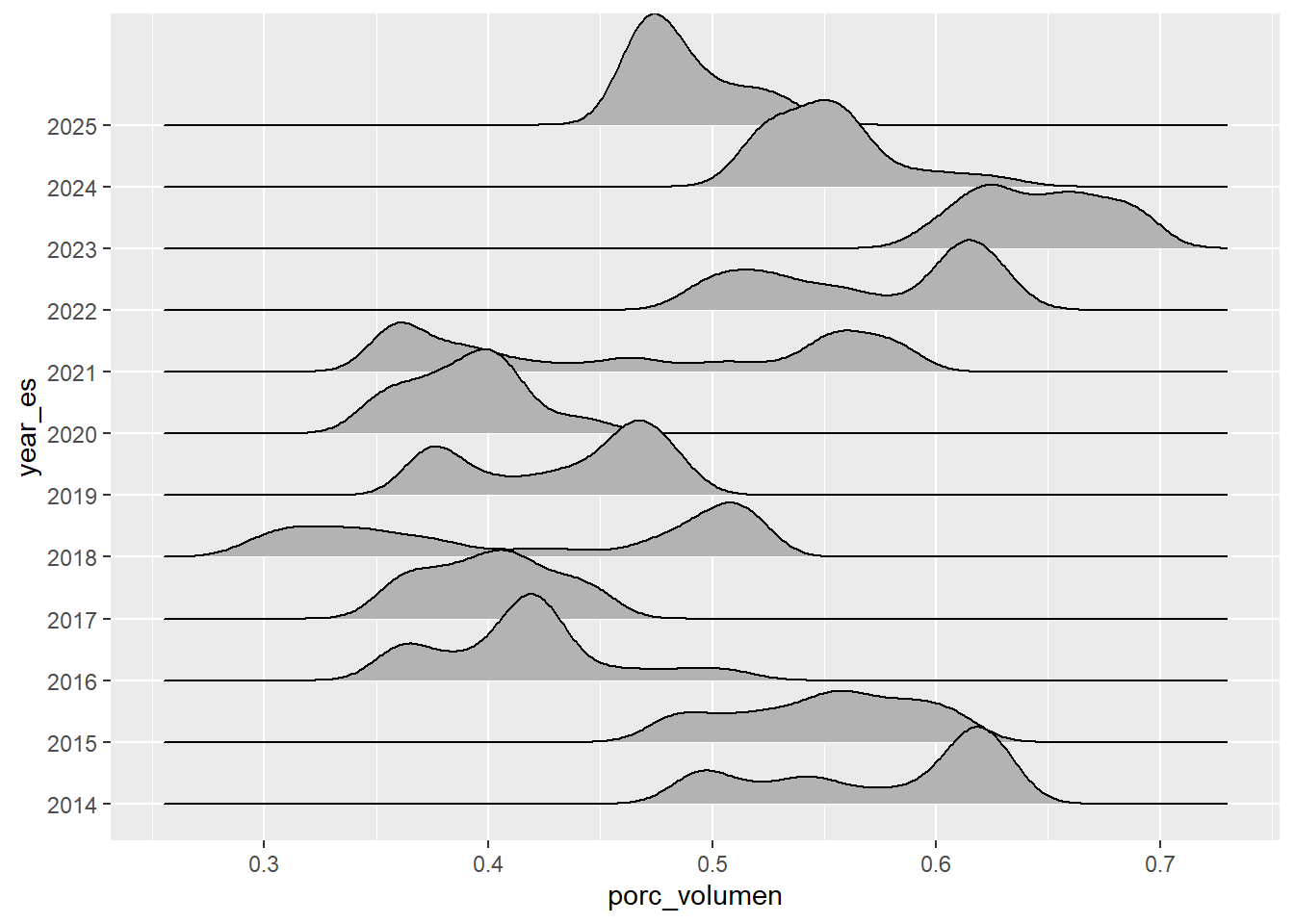

Code

df_embalses |> 
  filter(embalse == "AGREGADO BOGOTA") |> 
  mutate(year_es = as.factor(year_es),
         semestre = as.factor(semestre)) |> 
  ggplot(aes(x = porc_volumen, y = year_es, fill = semestre)) +
  geom_density_ridges()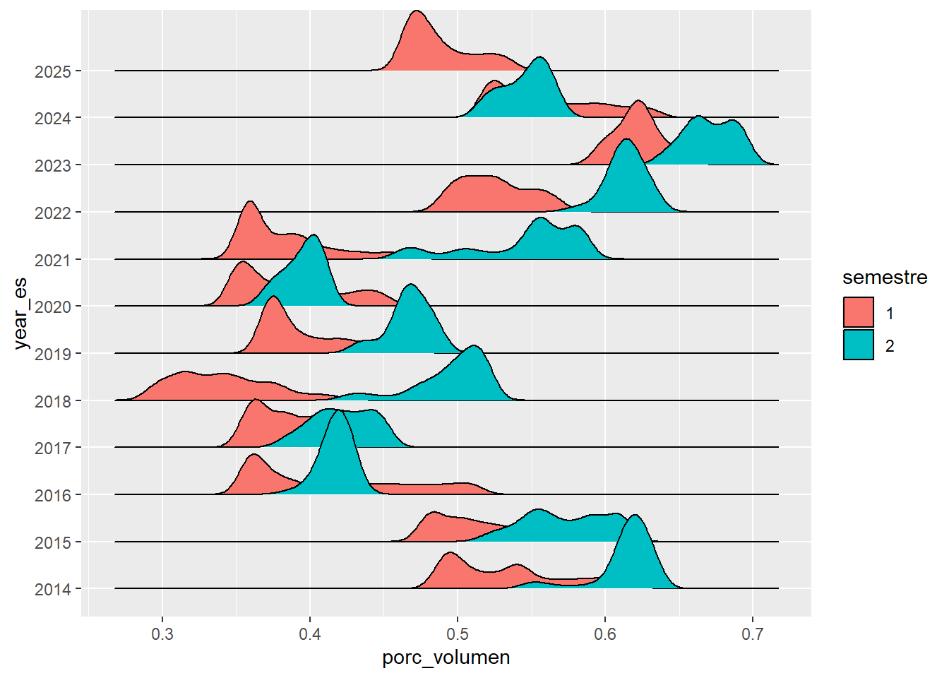

Coordenadas paralelas

Code

library(GGally)

df_embalses_resumen <-
  df_embalses |>
  group_by(embalse, year_es) |> 
  reframe(promedio = mean(porc_volumen, na.rm = TRUE)) |> 
  pivot_wider(names_from = embalse,
              values_from = promedio) |> 
  mutate(year_es = as.factor(year_es))


grafico_coordenadas <-
  ggparcoord(
  columns = 2:24, # variables numéricas
  groupColumn = 1, # variable categórica
  scale = "globalminmax", # Mantener las unidades originales
  data = df_embalses_resumen
) +
  theme(axis.text.x = element_text(angle = 45, hjust = 1))

grafico_coordenadas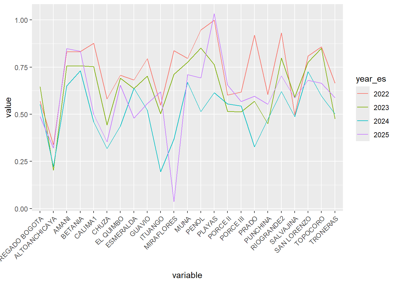

Code

ggplotly(grafico_coordenadas)

Donut

Code

resumen_creditos <-
  df_creditos |> 
  count(tipo_productor) |> 
  mutate(porcentaje = (n / sum(n)) * 100)

resumen_creditos$ymax <- cumsum(resumen_creditos$porcentaje)
resumen_creditos$ymin <- c(0, resumen_creditos$ymax[1:3])

# Agregar etiquetas con porcentajes
resumen_creditos <- resumen_creditos |>
  mutate(
    pos = (ymax + ymin) / 2,  # posición del texto
    etiqueta = paste0(tipo_productor, "\n", round(porcentaje, 1), "%")
  )

resumen_creditos |>
  ggplot(aes(
    ymax = ymax,
    ymin = ymin,
    xmax = 4,
    xmin = 3,
    fill = tipo_productor
  )) +
  geom_rect() +
  geom_text(aes(x = 3.5, y = pos, label = etiqueta),
            size = 3,
            fontface = "bold") +
  coord_polar(theta = "y") +
  xlim(c(1, 4)) +
  theme_void() +
  theme(legend.position = "none")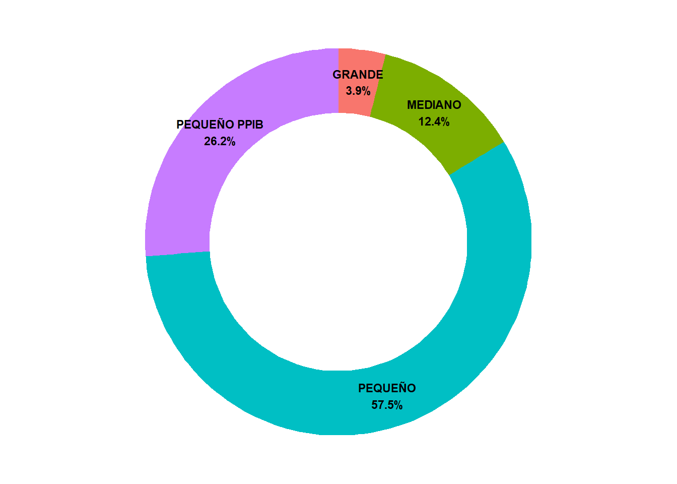

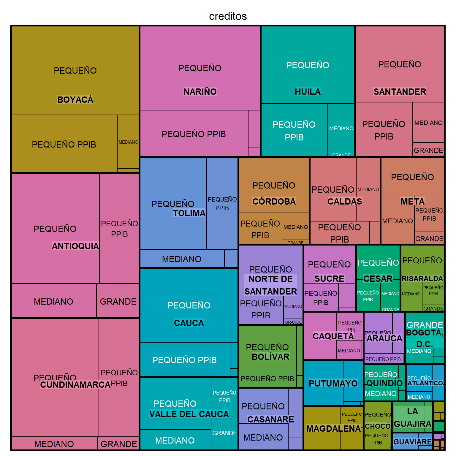
Treemap

Code

library(treemap)

resumen_creditos2 <-
  df_creditos |> 
  group_by(departamento_inversion, tipo_productor) |> 
  reframe(creditos = n(),
          total = mean(colocacion, na.rm = TRUE))

treemap(
  dtf = resumen_creditos2,
  index = c("departamento_inversion", "tipo_productor"),
  vSize = "creditos",
  type = "index"
)

Code

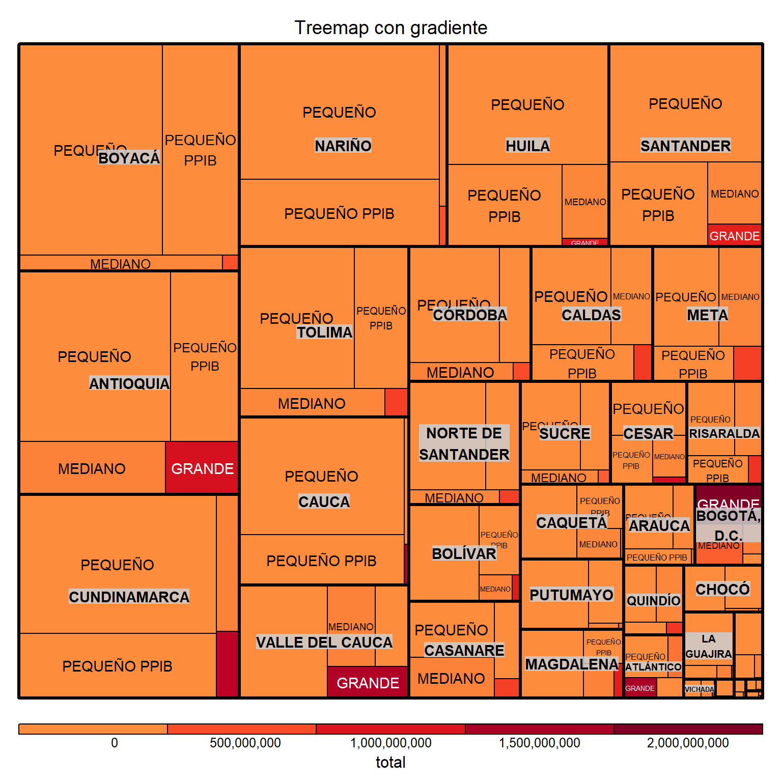
treemap(
  dtf = resumen_creditos2,
  index = c("departamento_inversion", "tipo_productor"),
  vSize = "creditos",
  vColor = "total",
  type = "value",
  palette = "YlOrRd",
  title = "Treemap con gradiente",
  format.legend = list(scientific = FALSE, big.mark = ","),
  n = 5
)

Mapa de calor

Code

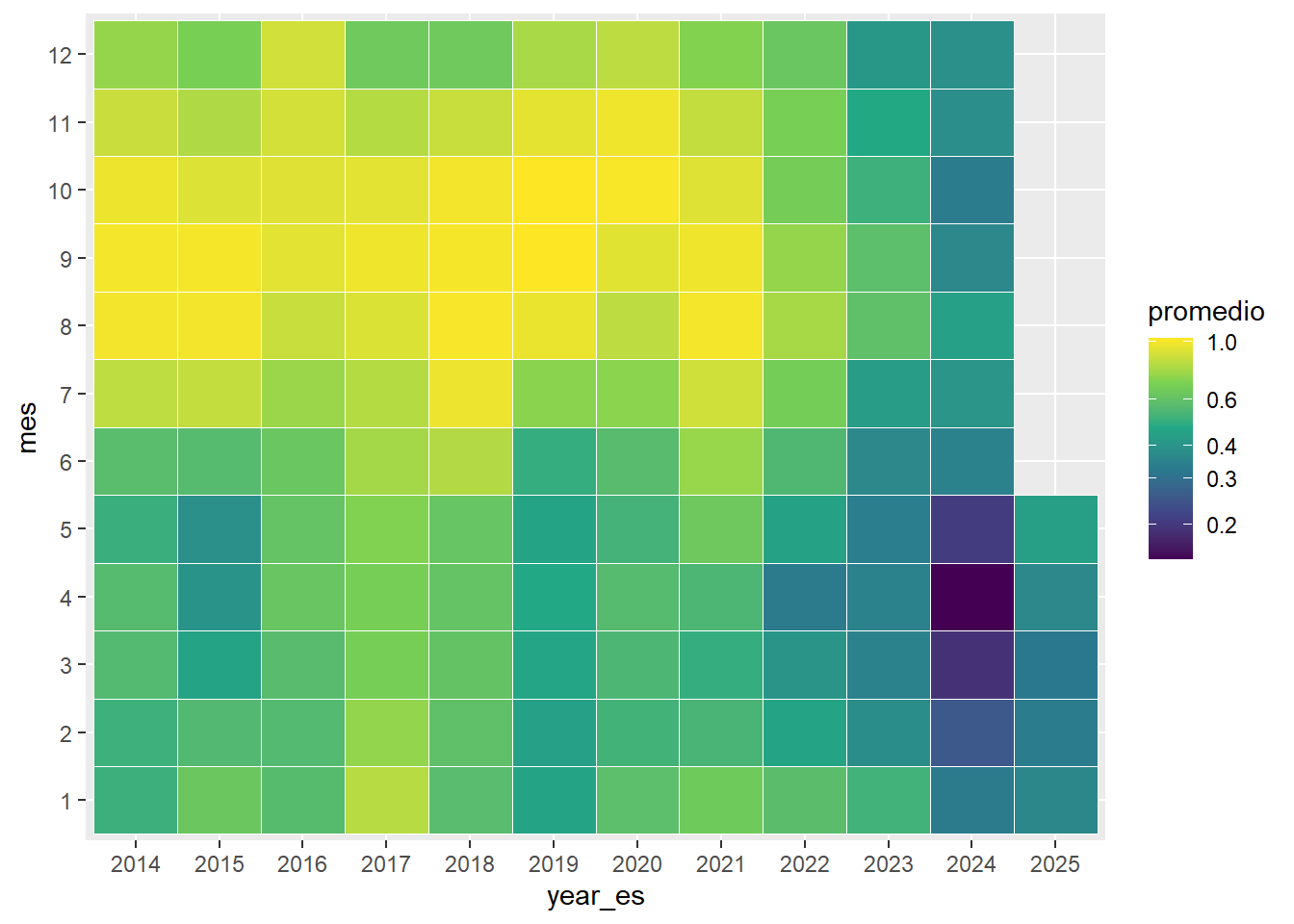
df_embalses |>
  filter(embalse == "CHUZA") |>
  group_by(year_es, mes) |>
  reframe(promedio = mean(porc_volumen, na.rm = TRUE)) |>
  mutate(year_es = as.factor(year_es),
         mes = as.factor(mes)) |>
  ggplot(aes(x = year_es, y = mes, fill = promedio)) +
  geom_tile(color = "white") +
  scale_fill_viridis_c()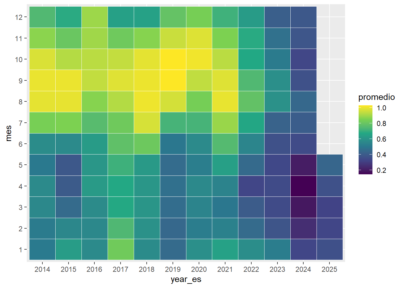

Code

library(scales)

df_embalses |>
  filter(embalse == "CHUZA") |>
  group_by(year_es, mes) |>
  reframe(promedio = mean(porc_volumen, na.rm = TRUE)) |>
  mutate(year_es = as.factor(year_es), mes = as.factor(mes)) |>
  ggplot(aes(x = year_es, y = mes, fill = promedio)) +
  geom_tile(color = "white") +
  scale_fill_viridis_c(trans = "log10",
                       breaks = trans_breaks(
                         trans = "log10",
                         inv = function(x)
                           round(10^x, digits = 1)
                       ))