Visualizaciones: mapas

Estadística

Author

Edimer David Jaramillo

Published

May 27, 2025

Bibliotecas

Code

library(tidyverse)
library(scales)
library(sf)
library(terra)
library(janitor)

Recursos importantes

Tipos de información geoespacial

Mapas

Code

mapa_depto <- st_read("datos/MGN2021_DPTO_POLITICO/MGN_DPTO_POLITICO.shp")

Reading layer `MGN_DPTO_POLITICO' from data source 
  `D:\UdeA\2025-01\estadistica\estadistica-202501\datos\MGN2021_DPTO_POLITICO\MGN_DPTO_POLITICO.shp' 
  using driver `ESRI Shapefile'
Simple feature collection with 33 features and 9 fields
Geometry type: MULTIPOLYGON
Dimension:     XY
Bounding box:  xmin: -81.73562 ymin: -4.229406 xmax: -66.84722 ymax: 13.39473
Geodetic CRS:  MAGNA-SIRGAS

Code

mapa_mpios <- st_read("datos/MGN2021_MPIO_POLITICO/MGN_MPIO_POLITICO.shp")

Reading layer `MGN_MPIO_POLITICO' from data source 
  `D:\UdeA\2025-01\estadistica\estadistica-202501\datos\MGN2021_MPIO_POLITICO\MGN_MPIO_POLITICO.shp' 
  using driver `ESRI Shapefile'
Simple feature collection with 1121 features and 12 fields
Geometry type: MULTIPOLYGON
Dimension:     XY
Bounding box:  xmin: -81.73562 ymin: -4.229406 xmax: -66.84722 ymax: 13.39473
Geodetic CRS:  MAGNA-SIRGAS

Mapa departamental

Code

mapa_depto |> 
  ggplot() +
  geom_sf()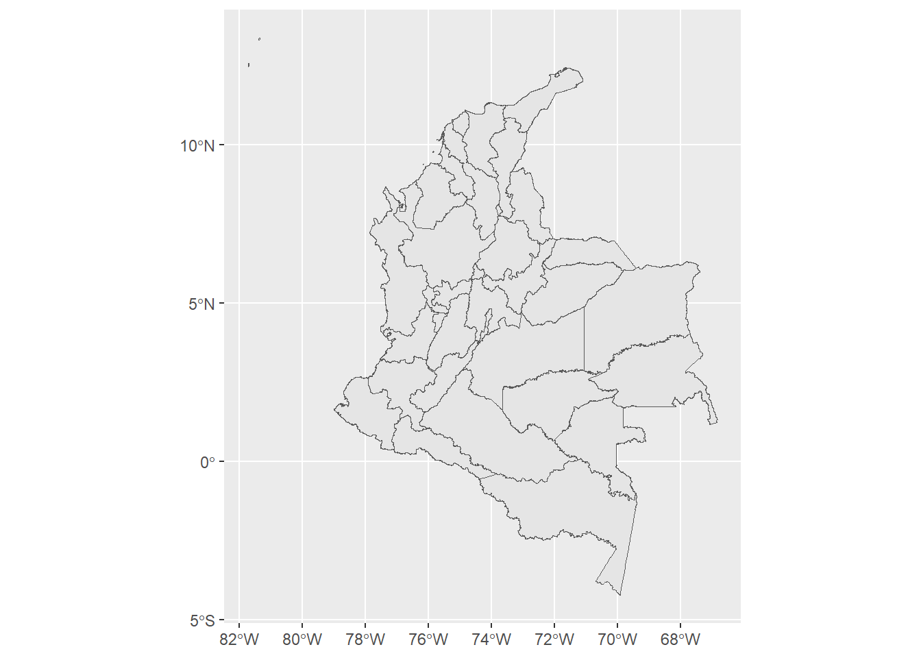

Mapa municipal

Code

mapa_mpios |> 
  ggplot() +
  geom_sf()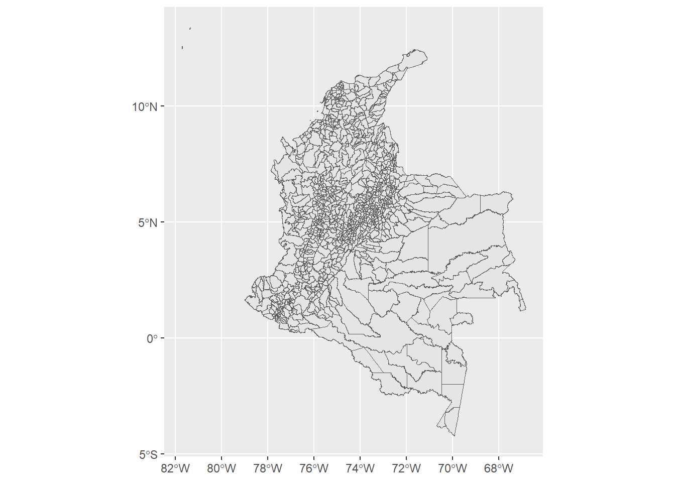

Podemos extraer un polígono (departamento o municipio) específico:

Code

mapa_mpios |> 
  filter(DPTO_CNMBR == "ANTIOQUIA") |> 
  ggplot() +
  geom_sf()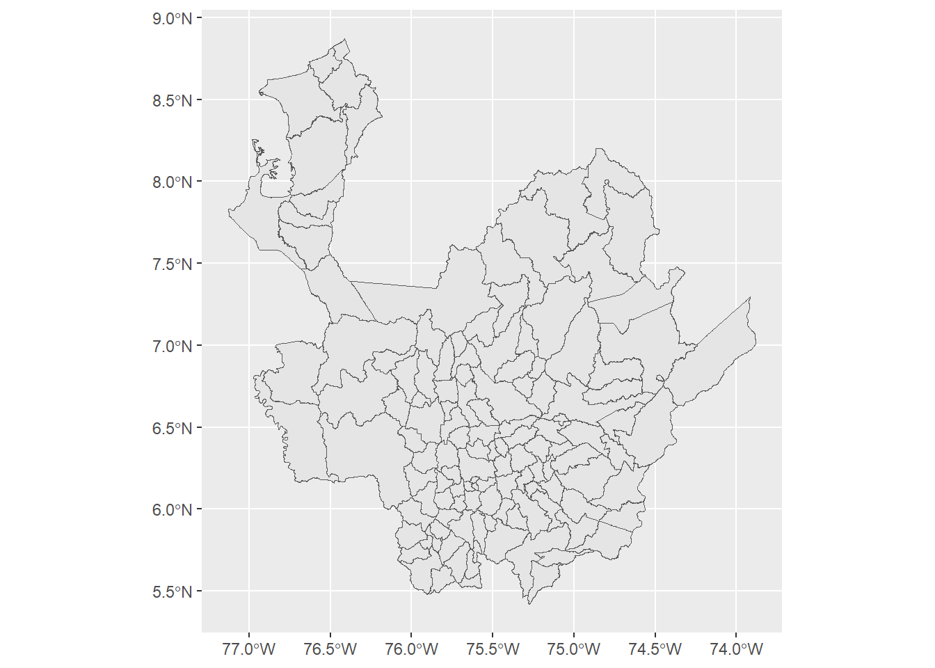

Créditos agropecuarios

Code

df_creditos <-
  read_csv("datos/Colocaciones_de_Cr_dito_Sector_Agropecuario_-_2021-_2024_20250502.csv") |> 
  clean_names()

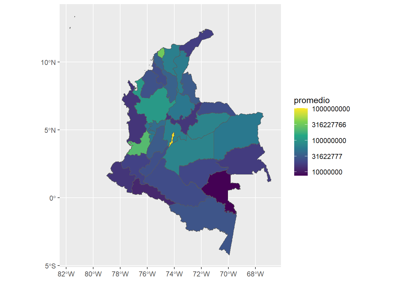
df_creditos |> head()

Resumimos a nivel de departamento para luego unir al mapa y graficar.

Code

df_resumen_deptos <-
  df_creditos |> 
  group_by(id_depto) |> 
  reframe(promedio = mean(colocacion, na.rm = TRUE))

mapa_deptos_creditos <-
  mapa_depto |>
  mutate(DPTO_CCDGO = as.numeric(DPTO_CCDGO)) |>
  left_join(df_resumen_deptos, df_creditos, by = c("DPTO_CCDGO" = "id_depto"))

mapa_deptos_creditos |>
  ggplot(aes(fill = promedio)) +
  geom_sf() +
  scale_fill_viridis_c(trans = "log10",
                       breaks = trans_breaks(
                         trans = "log10",
                         inv = function(x)
                           round(10 ^ x, digits = 1)
                       ))

Imagen raster

Code

raster_sg <- rast("datos/nitrogen_0-5cm_mean.tif")
raster_sg |> plot()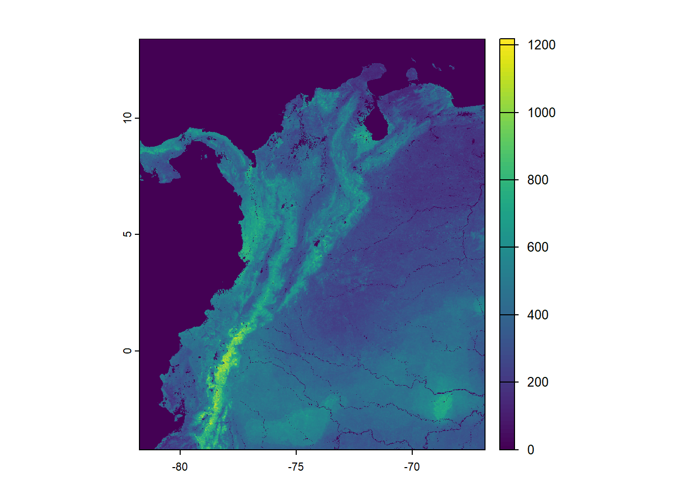

Extracción de datos para Colombia.

Code

capa_colombia <-
  raster_sg |> 
  mask(mapa_depto) |> 
  crop(mapa_depto)

Graficamos nuevamente la imagen raster:

Code

capa_colombia |> 
  plot()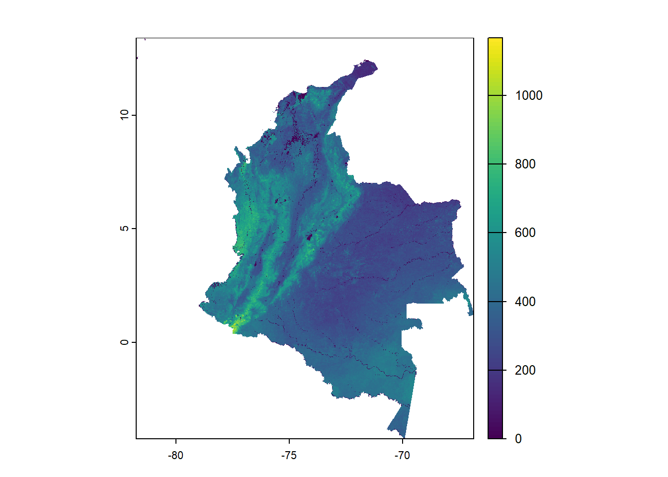

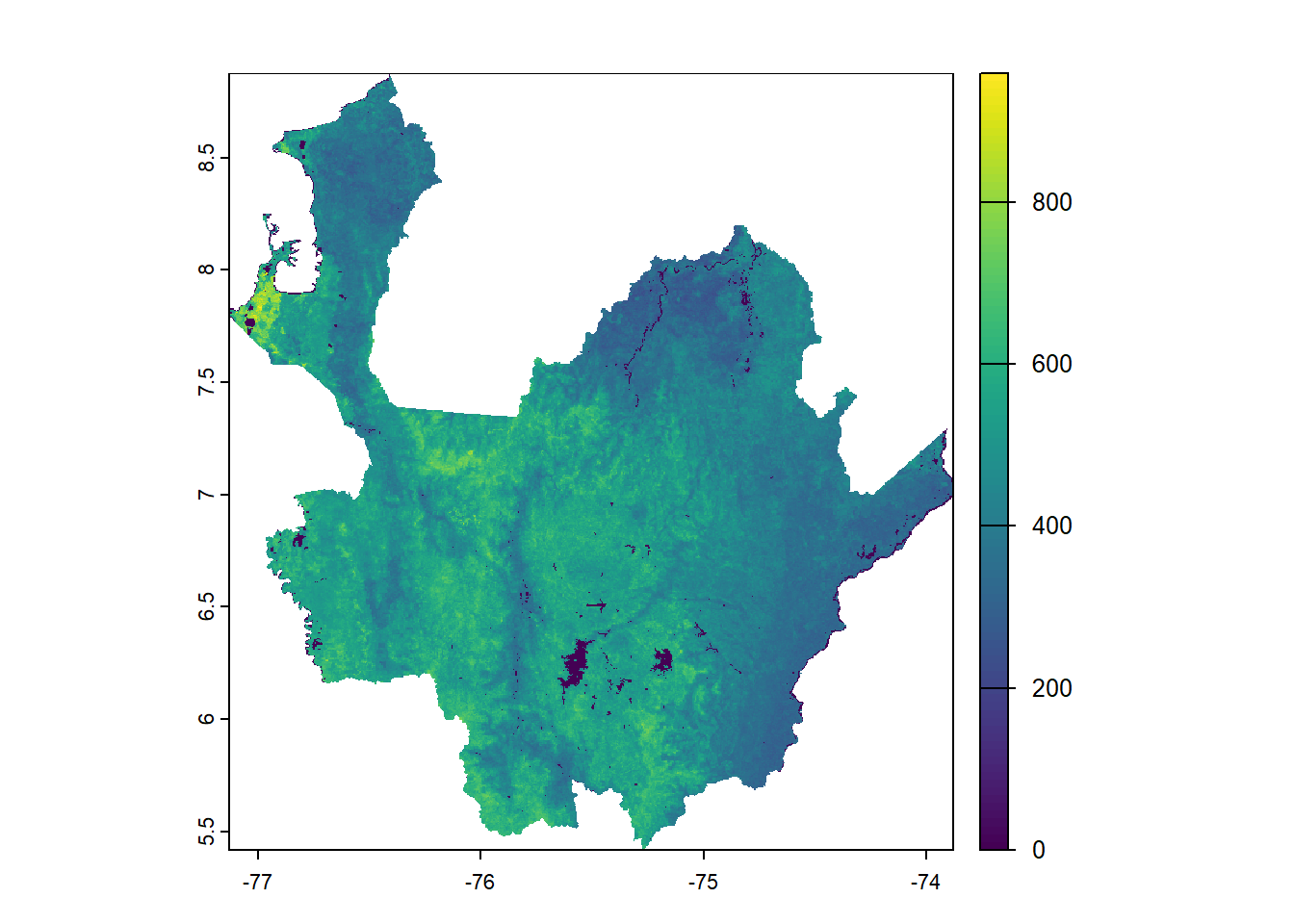
Podemos extraer la información desde un raster para un departamento o municipio específico:

Code

antioquia <- mapa_depto |> 
  filter(DPTO_CNMBR == "ANTIOQUIA")

capa_antioquia <-
  raster_sg |> 
  mask(antioquia) |> 
  crop(antioquia)

capa_antioquia |> plot()